This is the old vignette - you find the new vignette on CRAN: OneR vignette

Introduction

The following story is one of the most often told in the Data Science community: Some time ago the military built a system which aim it was to distinguish military vehicles from civilian ones. They chose a neural network approach and trained the system with pictures of tanks, humvees and missile launchers on the one hand and normal cars, pickups and trucks on the other. And after having reached a satisfactory accuracy they brought the system into the field (quite literally). It failed completely, performing no better than a coin toss. What had happened? No one knew, so they re-engineered the black box (no small feat in itself) and found that most of the military pics where taken at dusk or dawn and most civilian pics under brighter weather conditions. The neural net had learned the difference between light and dark!

Although this might be an urban legend the fact that it is so often told wants to tell us something:

1. Many of our Machine Learning models are so complex that we cannot understand them ourselves.
2. Because of 1. we cannot differentiate between the simpler aspects of a problem which can be tackled by simple models and the more sophisticated ones which need specialized treatment.

In one word: We need a good baseline which builds “the best simple model” that strikes a balance between the best accuracy possible with a model that is still simple to grasp: We have developed the OneR package for finding this sweet spot and thereby establishing a new baseline for classification models in Machine Learning.

This package is filling a longstanding gap because only a JAVA based implementation was available so far (RWeka package as an interface for the OneR JAVA class). Additionally several enhancements have been made (see below).

Design principles for the OneR package

The following design principles were followed for programming the package:

• Easy: The learning curve for new users should be minimal. Results should be obtained with ease and only minimal preprocessing and modeling steps should be necessary.
• Versatile: All types of data, i.e. categorical and numeric, should be computable - as input variable as well as as target.
• Fast: The running times of model trainings should be short.
• Accurate: The accuracy of trained models should be good overall.
• Robust: Models should not be prone to overfitting; the reached accuracy on training data should be comparable to the accuracy of predictions from new, unseen cases.
• Comprehensible: It should be easy to understand which rules the model has learned. Not only should the rules be easily comprehensible but they should serve as heuristics that are usable even without a computer.
• Reproducible: Because the used algorithms are strictly deterministic one will always get the same models on the same data. Many ML algorithms have stochastic components so that the data scientist will get a different model very time.
• Intuitive: Model diagnostics should be presented in form of a simple plot.
• Native R: The whole package is written in native R code. Thereby the source code can be easily checked and the whole package is very lean. Additionally the package has no dependencies at all other than base R itself.

The package is based on the – as the name might reveal – one rule classification algorithm [Holte93]. Although the underlying method is simple enough (basically 1-level decision trees, you can find out more here: OneR) several enhancements have been made:

• Missing values: In the original algorithm missing values were always handled as a separate level in the respective attribute. While missing values can sometimes reveal interesting patterns in other cases they are, well, just values that are missing. In the OneR package missing values can be handled as separate levels (level “NA”) or they can be omitted.
• Discretization of numeric data: The OneR algorithm can only handle categorical data so numeric data has to be discretized. The original OneR algorithm separates the respective values in ever smaller and smaller buckets until the best possible accuracy is being reached. In can be argued that this is the definition of overfitting and contradicts the original spirit of OneR because tons of rules (one for every bucket) will result. One can of course introduce a new parameter “maximum bucket size” but finding the right value for this one doesn’t come naturally either. Therefore, we take a radically different approach: There are several methods for handling numeric data in the package (in the bin and the optbin function), the most promising one is the “logreg” method in the optbin function which gives only as many bins as there are target categories and which optimizes the cut points according to pairwise logistic regressions. The performance of this method on several different datasets is very encouraging and the method will be explained in detail later.
• Tie breaking: Sometimes the OneR algorithm will find several attributes that provide rules which all give the same best accuracy. The original algorithm just took the first attribute. While this is implemented in the OneR function as the default too a different method for tie breaking can be chosen: The contingency tables of all “best” rules are tested against each other with a Pearson’s Chi squared test and the one with the smallest p-value is being chosen. The rationale behind this is that thereby the attribute with the best signal-to-noise ratio is being found.

Getting started with a simple example

You can also watch this video which goes through the following example step-by-step:

Install from CRAN and load package

install.packages("OneR")
library(OneR)

Use the famous Iris dataset and determine optimal bins for numeric data

data <- optbin(iris)

Build model with best predictor

model <- OneR(data, verbose = TRUE)
        
    Attribute    Accuracy
1 * Petal.Width  96%     
2   Petal.Length 95.33%  
3   Sepal.Length 74.67%  
4   Sepal.Width  55.33%  
---
Chosen attribute due to accuracy
and ties method (if applicable): '*'

Show learned rules and model diagnostics

summary(model)

Rules:
If Petal.Width = (0.0976,0.791] then Species = setosa
If Petal.Width = (0.791,1.63]   then Species = versicolor
If Petal.Width = (1.63,2.5]     then Species = virginica

Accuracy:
144 of 150 instances classified correctly (96%)

Contingency table:
            Petal.Width
Species      (0.0976,0.791] (0.791,1.63] (1.63,2.5] Sum
  setosa               * 50            0          0  50
  versicolor              0         * 48          2  50
  virginica               0            4       * 46  50
  Sum                    50           52         48 150
---
Maximum in each column: '*'

Pearson's Chi-squared test:
X-squared = 266.35, df = 4, p-value < 2.2e-16

Plot model diagnostics

plot(model)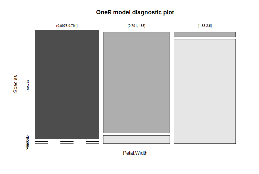

Use model to predict data

prediction <- predict(model, data)

Evaluate prediction statistics

eval_model(prediction, data)

           actual            
prediction   setosa versicolor virginica Sum
  setosa         50          0         0  50
  versicolor      0         48         4  52
  virginica       0          2        46  48
  Sum            50         50        50 150

           actual            
prediction   setosa versicolor virginica  Sum
  setosa       0.33       0.00      0.00 0.33
  versicolor   0.00       0.32      0.03 0.35
  virginica    0.00       0.01      0.31 0.32
  Sum          0.33       0.33      0.33 1.00

Accuracy:
0.96 (144/150)

Error rate:
0.04 (6/150)

Please note that the very good accuracy of 96% is reached effortlessly.

Petal.Width is identified as the attribute with the highest predictive value. The cut points of the intervals are found automatically (via the included optbin function). The results are three very simple, yet accurate, rules to predict the respective species:

If Petal.Width = (0.0976,0.791] then Species = setosa
If Petal.Width = (0.791,1.63]   then Species = versicolor
If Petal.Width = (1.63,2.5]     then Species = virginica

The nearly perfect separation of the colors in the diagnostic plot give a good indication of the model’s ability to separate the different species.

A more sophisticated real-world example

The next example tries to find a model for the identification of breast cancer. The example can run without further preparation:

library(OneR)

# http://archive.ics.uci.edu/ml/machine-learning-databases/breast-cancer-wisconsin/breast-cancer-wisconsin.names
# According to this source the best out-of-sample performance was 95.9%

# #  Attribute                     Domain
# -- -----------------------------------------
# 1. Sample code number           id number
# 2. Clump Thickness              1 - 10
# 3. Uniformity of Cell Size      1 - 10
# 4. Uniformity of Cell Shape     1 - 10
# 5. Marginal Adhesion            1 - 10
# 6. Single Epithelial Cell Size  1 - 10
# 7. Bare Nuclei                  1 - 10
# 8. Bland Chromatin              1 - 10
# 9. Normal Nucleoli              1 - 10
# 10. Mitoses                     1 - 10
# 11. Class:                      (2 for benign, 4 for malignant)

Load and name data

data <- read.csv("http://archive.ics.uci.edu/ml/machine-learning-databases/breast-cancer-wisconsin/breast-cancer-wisconsin.data", na.strings = "?")
data <- data[-1] #remove sample code number
class <- factor(data[ , ncol(data)], levels = c(2, 4), labels = c("benign", "malignant"))
data <- data[-ncol(data)]; data <- cbind(data, class)
names(data) <- c("Clump Thickness", "Uniformity of Cell Size", "Uniformity of Cell Shape", "Marginal Adhesion", "Single Epithelial Cell Size", "Bare Nuclei", "Bland Chromatin", "Normal Nucleoli", "Mitoses", "Class")

Divide training (80%) and test set (20%)

set.seed(123)
random <- sample(1:nrow(data), 0.8 * nrow(data))
data.train <- optbin(data[random, ])
Warning message:
In optbin(data[random, ]) :
  at least one instance was removed due to missing values
data.test <- data[-random, ]

Train OneR model on training set

model.train <- OneR(data.train, verbose = T)

    Attribute                   Accuracy
1 * Uniformity of Cell Size     92.83%  
2   Uniformity of Cell Shape    92.1%   
3   Bland Chromatin             90.99%  
4   Bare Nuclei                 90.44%  
5   Single Epithelial Cell Size 88.6%   
6   Normal Nucleoli             87.13%  
7   Marginal Adhesion           86.95%  
8   Clump Thickness             86.03%  
9   Mitoses                     78.68%  
---
Chosen attribute due to accuracy
and ties method (if applicable): '*'

Show model and diagnostics

summary(model.train)

Rules:
If Uniformity of Cell Size = (0.991,3.27] then Class = benign
If Uniformity of Cell Size = (3.27,10]    then Class = malignant

Accuracy:
505 of 544 instances classified correctly (92.83%)

Contingency table:
           Uniformity of Cell Size
Class       (0.991,3.27] (3.27,10] Sum
  benign           * 344        10 354
  malignant           29     * 161 190
  Sum                373       171 544
---
Maximum in each column: '*'

Pearson's Chi-squared test:
X-squared = 381.11, df = 1, p-value < 2.2e-16

Plot model diagnostics

plot(model.train)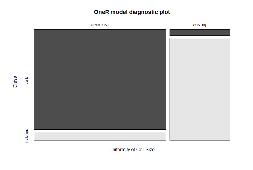

Use trained model to predict test set

prediction <- predict(model.train, data.test)

Evaluate model performance on test set

eval_model(prediction, data.test)

           actual           
prediction  benign malignant Sum
  benign        90         8  98
  malignant      1        41  42
  Sum           91        49 140

           actual           
prediction  benign malignant  Sum
  benign      0.64      0.06 0.70
  malignant   0.01      0.29 0.30
  Sum         0.65      0.35 1.00

Accuracy:
0.9357 (131/140)

Error rate:
0.0643 (9/140)

The best reported accuracy on this dataset was at 97.5% and it was reached with considerable effort. The reached accuracy for the test set here lies at 93.6%! This is achieved with the following two simple rules:

## If Uniformity of Cell Size = (0.991,3.27] then Class = benign
## If Uniformity of Cell Size = (3.27,10]    then Class = malignant

Uniformity of Cell Size is identified as the attribute with the highest predictive value. The cut points of the intervals are again found automatically (via the included optbin function). The very good separation of the colors in the diagnostic plot give a good indication of the model’s ability to differentiate between benign and malignant tissue.

Included functions

• OneR is the main function of the package: builds a model according to the One Rule machine learning algorithm for categorical data. All numerical data is automatically converted into five categorical bins of equal length. When verbose is TRUE it gives the predictive accuracy of the attributes in decreasing order.
• bin discretizes all numerical data in a dataframe into categorical bins of equal length or equal content.
• optbin discretizes all numerical data in a dataframe into categorical bins where the cut points are optimally aligned with the target categories, thereby a factor is returned. When building a OneR model this could result in fewer rules with enhanced accuracy. The cutpoints are calculated by pairwise logistic regressions (method "logreg") or as the means of the expected values of the respective classes ("naive"). The function is likely to give unsatisfactory results when the distributions of the respective classes are not (linearly) separable. Method "naive"should only be used when distributions are (approximately) normal, although in this case "logreg" should give comparable results, so it is the preferable (and therefore default) method.
• eval_model is a simple function for evaluating a OneR classification model, which is included in the package for convenience reasons. It prints prediction vs. actual in absolute and relative numbers. Additionally, it gives the accuracy and error rate. The second argument actual is a dataframe which contains the actual data in the last column. A single vector is allowed too.
• maxlevels removes all columns of a dataframe where a factor (or character string) has more than a maximum number of levels. Often categories that have very many levels are not useful in modelling OneR rules because they result in too many rules and tend to overfit. Examples are IDs or names.

Help overview

help(package = OneR)

...or as a pdf here: OneR.pdf

Sources

[Holte93] R. Holte: Very Simple Classification Rules Perform Well on Most Commonly Used Datasets, 1993. Available: http://www.mlpack.org/papers/ds.pdf.

Contact

I would love to hear about your experiences with the OneR package. Please drop me a note - you can reach me at my university account: Holger K. von Jouanne-Diedrich

License

This package is under MIT License.